Researchers are often interested in investigating how the prevalence of topics change over time. The keyATM can use time stamps for the prior for document-topic distribution through Hidden Markov Model (Chib 1998).
Section 4 of Eshima et al. (2024) explains the dynamic keyATM in details. As explained in keyATM Covariates, we recommend researchers to construct a numeric or an integer vector of time stamps after preprocessing texts.
Preparing time index
Please read Preparation for the reading of documents and creating a list of keywords.
We use the US Presidential inaugural address data we prapared (documents and keywords).
##   Year  President FirstName                 Party
## 1 1789 Washington    George                  none
## 2 1793 Washington    George                  none
## 3 1797      Adams      John            Federalist
## 4 1801  Jefferson    Thomas Democratic-Republican
## 5 1805  Jefferson    Thomas Democratic-Republican
## 6 1809    Madison     James Democratic-Republican
# Divide by a decade
# Timestamp should start with 1 (the variable "Period")
vars %>%
  as_tibble() %>%
  mutate(Period = (vars$Year - 1780) %/% 10 + 1) -> vars_period
vars_period %>% select(Year, Period)
## # A tibble: 58 × 2
## Year Period
## <int> <dbl>
## 1 1789 1
## 2 1793 2
## 3 1797 2
## 4 1801 3
## 5 1805 3
## 6 1809 3
## 7 1813 4
## 8 1817 4
## 9 1821 5
## 10 1825 5
## # ℹ 48 more rowsThe time index (Period) should start from 1
and increment by 1 (ascending order). To properly process date, please
consider using the lubridate package.
We pass the time index to the keyATM() function,
specifying the number of hidden states with the num_states
in the model_settings argument.
out <- keyATM(
  docs = keyATM_docs,
  no_keyword_topics = 3,
  keywords = keywords,
  model = "dynamic",
  model_settings = list(
    time_index = vars_period$Period,
    num_states = 5
  ),
  options = list(seed = 250)
)
Once you fit the model, you can save the model with
saveRDS() for replication. This is the same as the base model.
You can resume the iteration by specifying
the resume argument.
Interpreting results
We can use the interpretation functions, such as
top_words(), top_docs(),
plot_modelfit(), as in the base keyATM.
top_words(out)## 1_Government 2_Congress 3_Peace 4_Constitution 5_ForeignAffairs
## 1 government national world [✓] constitution [✓] country
## 2 states great new union united
## 3 public congress [✓] nation power every
## 4 laws [✓] political freedom [✓] rights [✓] war [✓]
## 5 law [✓] made america people nations
## 6 citizens policy let now foreign [✓]
## 7 one support time duty free
## 8 interests party [✓] peace [✓] present principles
## 9 state time one general duties
## 10 powers office government interest just
## Other_1 Other_2 Other_3
## 1 liberty right people
## 2 work many great
## 3 hope much good
## 4 every progress men
## 5 long ever spirit
## 6 citizens yet justice
## 7 strength secure never
## 8 believe order american
## 9 fellow take first
## 10 land responsibility futureSince each state has a unique prior for the document-topic
distributions, the plot_alpha() function produces a
different figure from the base
keyATM.
fig_alpha <- plot_alpha(out)
fig_alpha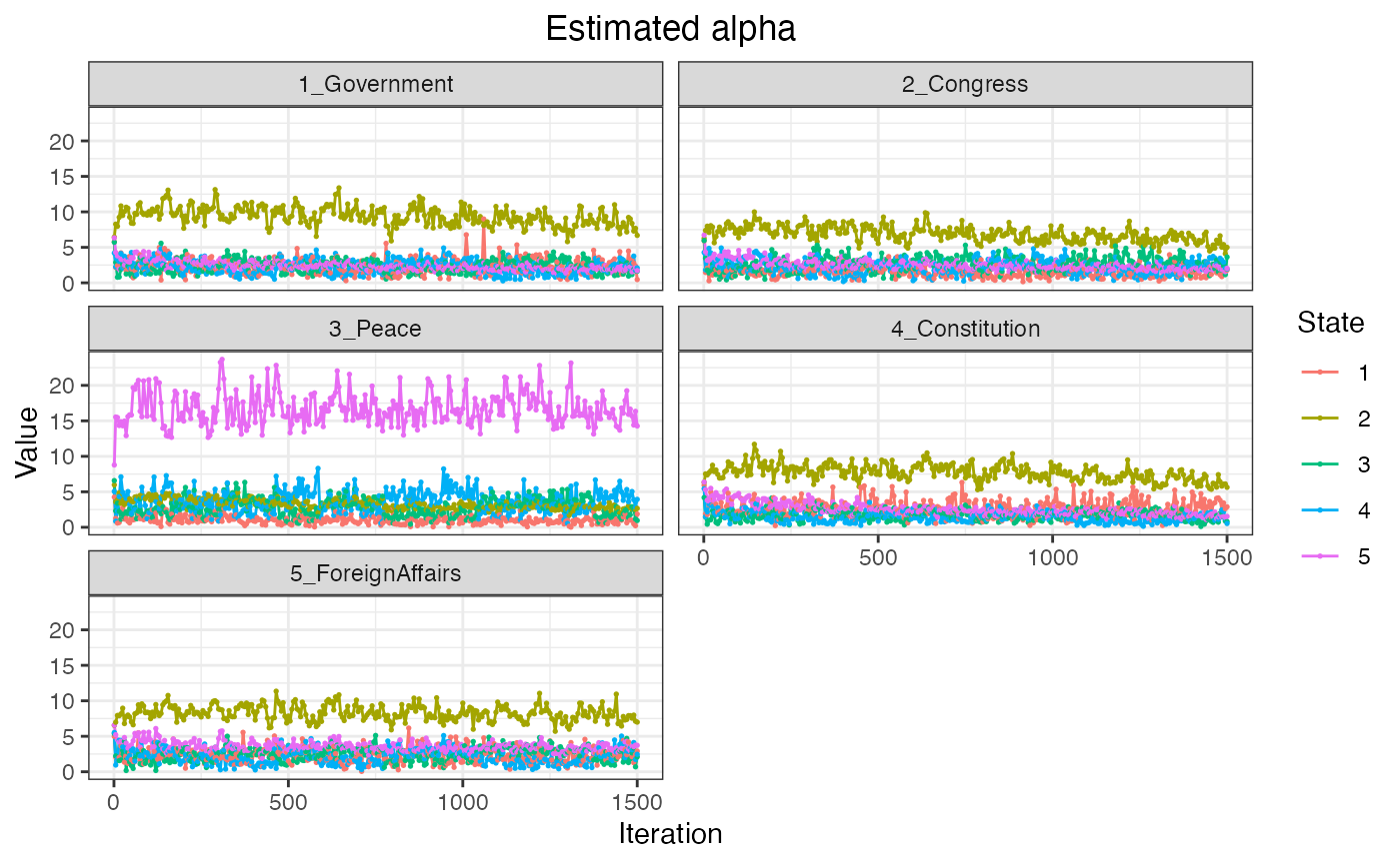
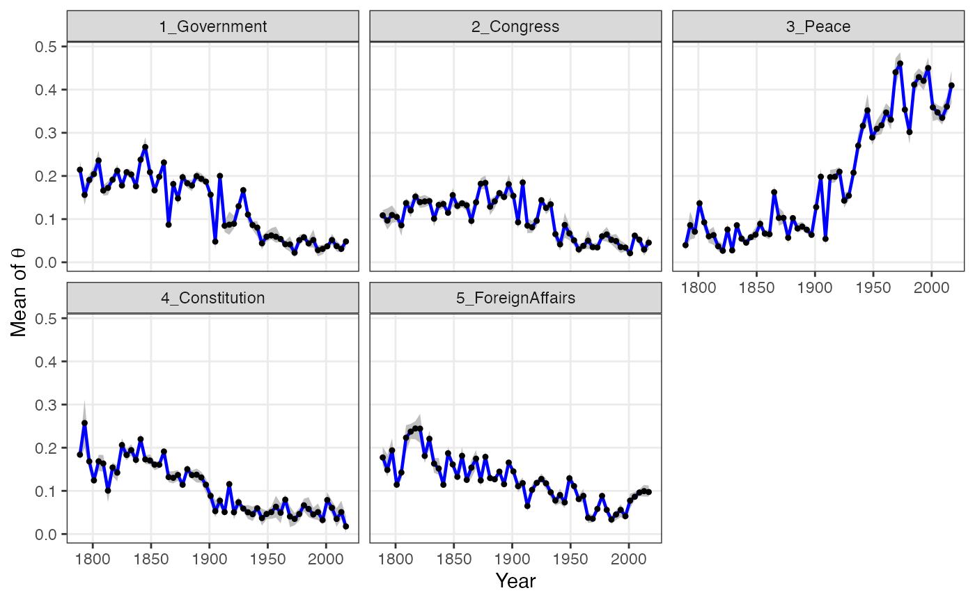
Finally, we can plot the time trend of topics with the
plot_timetrend() function. With the
time_index_label argument, you can label each time index.
Note that store_theta option in the keyATM()
function should be TRUE to show 90% credible intervals.
out <- keyATM(
  docs = keyATM_docs,
  no_keyword_topics = 3,
  keywords = keywords,
  model = "dynamic",
  model_settings = list(
    time_index = vars_period$Period,
    num_states = 5
  ),
  options = list(seed = 250, store_theta = TRUE, thinning = 5)
)
fig_timetrend <- plot_timetrend(out, time_index_label = vars$Year, xlab = "Year")
fig_timetrend